Introduction
I can still remember the moment when I created a LinkedIn profile. The act felt almost defiant as it meant that I was going to leave the sheltered student life behind me. Little did I know that ten years from that moment I would be writing a blog about the event broker system powering the social media platform, and then creating an event about it on the very same platform. Neither did I know that the system in question had the name Apache Kafka or that it would such a success story among technology companies after its inception at LinkedIn.
Shortly put, the Apache Kafka platform provides an open-source solution for building event-driven software. This in turn allows companies to get a systematic and almost real-time view of their data which is immensely valuable. Mind you, one crucial aspect of the Chernobyl disaster was that it took almost 30 minutes for the sensor data from the nuclear reactor to reach the monitors of the operators.
I was first introduced to Apache Kafka sometime in 2018 but did not get to use the platform back in the day. I was a mobile app developer of sorts. However, fast forward to today and Apache Kafka is all the rage at work. As I wanted to get a better grasp of it, I decided to do what I have always done — a demo project that explores the technology that interests me. Namely, I wanted to create a piece of software that demonstrates how Kafka event streams can be composed and how “business domain” concepts can be mapped to Kafka topics and their partitions.
This blog is similar to JSON lines for fun and profit from last year in that I present a walk-through of a simple codebase. In a way, this is also a logical sequel to the blog since I now pick off from the conclusion of the blog. Capturing the event stream of a piece of software can be exploited to construct novel pieces of software.
Central Limit Theorem
The inspiration for the demo project for this blog came from “attending” “Probabilistic Systems Analysis and Applied Probability,” an open university course from MIT. I am simply lost for words when thinking about the intellectual depth of probability theory and its philosophical implications. In particular, one of the most fascinating results discussed on the course is the Central Limit Theorem (CLT) that the lecturer, Prof. John Tsitsiklis, presents here.
I encourage you watch the whole course in order to understand what CLT strictly speaking means because there are a lot of nitty-gritty details. I will deliberately cut some corners and state that it explains why it is a good approximation to assume that the randomness observed in a dataset is distributed normally, i.e. the distribution follows the familiar bell curve shape.
The thinking behind CLT is that when a stochastic process involves averaging n random variables, the resulting distribution of the averages converges to a normal distribution as n tends to infinity. The proof is non-trivial and beyond the scope of this blog. However, the profound aspect of CLT is its generality. It matters not what the distribution of the original random variables is (exponential, binomial, uniform, …) nor how skewed it is.
Different distributions have different rates of convergence; a particularly striking example can be constructed when the samples have a binomial distribution. This kind of an averaging process can be demonstrated with a so-called Galton board (see the attached video) that the candid reader might recall from high school.
At the risk of veering off to a tangent, I would like to nonetheless emphasize the philosophical lesson that the CLT has to offer. When we flip the Galton board experiment around and state that we observed a normal distribution, it is basically hard evidence that the underlying phenomenon is figuratively made of a swarm of bouncing beads, each following their own complex and random trajectory. When understood fully, the CLT lets us better appreciate the complexity of the processes going on inside our cells, craniums or in the nether region of our bodies. It instructs us to avoid simplistic reasoning that is the bane of our identity-politics ridden time.
The idea
With the theory and polemic out of my chest, let’s turn our attention to code. I will assume that you already have some familiarity with Apache Kafka so that I will not go over the mechanics of setting up the development environment or the basic concepts of Kafka topics and streams.
What we will build is a kind of a Galton board. We will start with a process
that sends an indefinite stream of pseudorandom numbers to a Kakfa topic called
samples. Think of it as a simulated sensor of some device that measures values
with a fixed frequency, every 500 milliseconds say. The samples will be from the
standard uniform distribution.
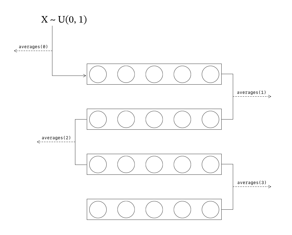
We will then feed the samples to an averaging process with a fixed sample size. In the attached diagram, this number would be five. As the resulting stream is again a stream of random numbers, we can feed it as input to the averaging process back again.
The resulting average numbers will be published in a separate topic which will be consumed by the application for an eyeball statistical analysis. That is, the numbers originating from different levels of averaging can be separately plotted as histograms. The hypothesis is that the more rounds of averaging for a particular number, the closer it should be to a real normal deviate.
For an averaging depth of k, one could naively create k topics named
averages0, averages1 and so on. However, I want to limit myself to a single
topic called averages with a configurable number of partitions, one for each
averaging level. This way, this piece of “domain logic” is elegantly encoded in
the structure of the Kafka topic itself.
If it takes N samples to compute an average, a number at partition k is made of Nk of the original uniform random numbers as you can deduce from the attached diagram. In particular, partition 0 maps to the original non-averaged samples. As an aside, I suppose this is not a very clever way to approach partitioning for a production system as the load per partition varies exponentially.
A skeleton
For an overview of the walk-through, the finished code will have the following layout:
.
├── docker-compose.yaml
├── pom.xml
└── src
    └── main
        ├── java
        │   └── net
        │       └── keksipurkki
        │           └── demos
        │               ├── Application.java
        │               ├── Histogram.java
        │               ├── kafka
        │               │   ├── AveragesProducer.java
        │               │   ├── Config.java
        │               │   ├── SamplesProducer.java
        │               │   └── Topics.java
        │               └── ws
        │                   ├── HistogramMessage.java
        │                   └── WebSocketConfig.java
        └── resources
            ├── application.properties
            ├── logback.xml
            └── static
                ├── app.js
                ├── favicon.ico
                ├── index.html
                └── styles.css
Let’s start with the Kafka setup for the Topics:
@Configuration
@EnableConfigurationProperties(Topics.TopicProperties.class)
public class Topics {

    private final TopicProperties props;

    public Topics(TopicProperties props) {
        this.props = props;
    }

    @Bean
    public NewTopic samplesTopic() {
        return TopicBuilder.name(props.samples())
            .partitions(1)
            .compact()
            .build();
    }

    @Bean
    public NewTopic averagesTopic(int partitions) {
        return TopicBuilder.name(props.averages())
            .partitions(partitions)
            .compact()
            .build();
    }

    @ConfigurationProperties(prefix = "app.topics")
    public record TopicProperties(String samples, String averages) {

    }

}
The reader will recognize that I am using Spring to wire
the application together. The samples topic can then be injected to
SamplesProducer:
@Component
public class SamplesProducer {

    private final NewTopic samplesTopic;
    private final KafkaTemplate<UUID, Double> template;

    public SamplesProducer(NewTopic samplesTopic, KafkaTemplate<UUID, Double> template) {
        this.samplesTopic = samplesTopic;
        this.template = template;
    }

    public Runnable measurement() {
        // A simulated sensor device
        final var topic = samplesTopic.name();
        final Supplier<Double> sensor = ThreadLocalRandom.current()::nextDouble;

        return () -> {
            template.send(topic, UUID.randomUUID(), sensor.get());
        };
    }
}
and we can “start the measurement” like so:
@SpringBootApplication
@EnableScheduling
public class Application {

    private final Runnable measurement;

    Application(SamplesProducer producer) {
        this.measurement = producer.measurement();
    }

    public static void main(String... args) {
        var app = new SpringApplication(Application.class);
        app.run(args);
    }

    @Scheduled(fixedRateString = "${app.samples.rate.millis}")
    void measureSamples() {
        measurement.run();
    }
}
The resulting stream of numbers will have the type of
Double.
If you are not a programmer or just starting your journey, the term may be
confusing. It refers to double-precision. A single-precision stream of numbers
could be achieved by calling ThreadLocalRandom::nextFloat.
An additional thing to emphasize about the code so far is that generating
pseudorandom numbers is trickier than you might think. We have hopefully
sidestepped any of the potential problems by using the ThreadLocalRandom class
from the JDK, as advised by Joshua Bloch in
Effective Java
(Item 59).
Another point worthy of mentioning is that I limited myself to the standard uniform distribution to keep things simple. A neat fact about pseudorandom number generation is that there is a way to massage the uniform distribution to any distribution of your liking with the help of a technique known as Inverse transform sampling. If I wanted to have normally distributed random numbers without this Galton board business, I could go shopping for a formula and use that. However, for the special and highly important case of normal deviates, there are algorithms that are computationally more efficient than the inverse transform method, the Box-Muller transform being arguably the most famous of them.
Now, a skeletal implementation of the AveragesProducer that consumes samples
and averages them could look like this:
@Slf4j
@Component
public class AveragesProducer {

    private final NewTopic samplesTopic;
    private final NewTopic averagesTopic;

    AveragesProducer(NewTopic samplesTopic, NewTopic averagesTopic) {
        this.samplesTopic = samplesTopic;
        this.averagesTopic = averagesTopic;
    }

    public KStream<UUID, Double> stream(StreamsBuilder builder) {
        var sampleSize = 2;

        var result = builder.<UUID, Double>stream(samplesTopic.name());
          .process(() -> new DoubleAggregator(sampleSize))
          .mapValues((_, doubles) -> DoubleStream.of(doubles).average().orElseThrow())

        result.to(averagesTopic.name());

        return result;
    }

    private static class DoubleAggregator implements Processor<UUID, Double, UUID, double[]> {
        private final ArrayList<Double> values;
        private final int size;
        private ProcessorContext<UUID, double[]> context;

        DoubleAggregator(int size) {
            this.size = size;
            this.values = new ArrayList<>();
        }

        @Override
        public void init(ProcessorContext<UUID, double[]> context) {
            this.context = context;
        }

        @Override
        public void process(Record<UUID, Double> record) {
            if (values.size() >= size) {
                var array = values.stream().mapToDouble(Double::doubleValue).toArray();
                context.forward(record.withValue(array));
                values.clear();
            }
            values.add(record.value());
        }
    }

}
There is a lot going on in this class. Hopefully you can nonetheless grasp how
the DoubleAggregator processes double values and outputs arrays of doubles
whenever the sampleSize limit has been reached. The average value of the array
can then be computed with DoubleStream.of(values).average().orElseThrow(). The
DoubleStream interface comes from the
Java Stream API,
giving the end result that authentic over-engineered feel. I beg the reader to
allow the author his indulgences.
Finally, the last piece of plumbing is to consume the averages topic. Thanks to
Spring Kafka, setting up the
machinery is as easy as annotating a method with the @KafkaListener
annotation. I reckon the Application class is as good a place as any to stick
in the following lines of code:
    // Application.java

    @KafkaListener(topics = "${app.topics.averages}", groupId = "averages")
    void onReceiveAverage(ConsumerRecord<UUID, Double> average) {
        log.info("Received an average. AveragingLevel = {}, Value = {}", average.partition(), average.value());
    }
Stream composition
The next step is generalize what we have built so far. That is, we need to somehow use the fact that we have allocated a number of partitions for the averages topic and somehow re-average the averages. To be honest with you, I am cheating a little bit. Like a television chef that puts a tray of cookies in the oven just to pull a previously made batch from under the counter, the setup I showed you so far is just right for demonstrating how stream composition works.
I spent a good while reading the docs and there were a couple of false starts which are inevitable when learning something new. In particular, it helped me to realize that the Kafka Streams library provides a high-level API for manipulating Kafka topics as streams and you need to declare the library as a dependency explicitly when using the Spring Kafka framework.
Long story short, we only need to adjust the AveragesProducer a little bit to
achieve what we want:
    public KStream<UUID, Double> stream(StreamsBuilder builder) {
        var result = builder.<UUID, Double>stream(samplesTopic.name());

        final var levelDepth = averagesTopic.numPartitions();
        final var sampleSize = 2;

        log.info("Configuring a stream for sample averaging. Depth = {}, SampleSize = {}", levelDepth, sampleSize);

        // Averaging level = 0 == no averaging
        result.to(averagesTopic.name(), fixedPartition(0));

        for (var partition = 1; partition < levelDepth; partition++) {
            log.trace("Configuring stream topology for partition {}", partition);

            final int level = partition + 1;

            result = result
                .process(() -> new DoubleAggregator(sampleSize))
                .peek((_, v) -> log.debug("Level = {}. Got a sample of length {}", level, v.length))
                .mapValues((_, v) -> DoubleStream.of(v).average().orElseThrow())
                .peek((_, v) -> log.debug("Level = {}. Average = {}", level, v));

            result.to(averagesTopic.name(), fixedPartition(partition));
        }

        return result;
    }

    private Produced<UUID, Double> fixedPartition(int partition) {
        return Produced.streamPartitioner((_, _, _, _) -> partition);
    }
Pretty neat, aye? I hope the code is so readable that it explains itself. The
only thing I want to emphasize is the fixedPartition(int partition) method
that returns a Produced object from the Kafka streams library. It is used to
tell Kafka to forgo its default partitioning logic and instead send the numbers
to the partition that I tell it.
The static Procuced.streamPartitioner method wants a
StreamPartitioner.
Its explicit interface would be:
interface StreamPartitioner<K, V> {
  Integer partition(String topic, K key, V value, int numPartitions)
}
However, it turns out I can make use of a recent change in
Java syntax
and ignore all the formal parameters by naming them with an underscore _. It
may look weird at first, but this is actually a really welcome change as it
codifies an age-old convention originating in the functional programming camp.
I do not even know exactly why my little lambda solution works, and I guess this is specifically the objective of the recent changes in Java language design. Long gone are the days when you would have needed to instantiate an object that implements this interface with the boilerplate and ceremony that Java is infamous for. So far I have been really liking how smart the Java compiler has become, and I bet the wizards in the Java committees have done their homework in order to avoid the fate of C++ as a language that is syntactically just too “rich.”
Visualization
We can now turn our attention to the data that AveragesProducer sends to
Application. To aggregate the averages per partition, we introduce a simple
class representing a histogram:
public class Histogram {

    private final BigDecimal min;
    private final BigDecimal max;
    private final BigDecimal delta;
    private final int[] counts;
    private final int id;

    public Histogram(int id, int numBins, double min, double max) {
        Assert.isTrue(min < max, "Min < Max!");
        Assert.isTrue(numBins > 0, "numBins must be a positive number");
        this.id = id;
        this.counts = new int[numBins]; // zeros
        this.min = new BigDecimal(min).setScale(2, HALF_DOWN);
        this.max = new BigDecimal(max).setScale(2, HALF_DOWN);
        this.delta = this.max.subtract(this.min);
    }

    public void record(Double value) {
        if (value >= max.doubleValue() || value < min.doubleValue()) {
            log.warn("Ignoring value {}. Out of range", value);
            return;
        }
        counts[bin(value)]++;
    }

    private int bin(double value) {
        return (int) Math.floor(counts.length * (value - min.doubleValue()) / this.delta.doubleValue());
    }


    public static Histogram newHistogram(int level) {
        return new Histogram(level, 10, 0.0d, 1.0d);
    }
}
The code is simplified in the sense that the factory method hardcodes the number of bins and data range to 10 and [0, 1). In a real application we would need more flexibility, and these values would need to be determined from the data itself.
The Application can then be modified to record the averages to a map of
histograms where the key is the partition number:
    private final Map<Integer, Histogram> histograms = new ConcurrentHashMap<>();

    @KafkaListener(topics = "${app.topics.averages}", groupId = "averages")
    void onReceiveAverage(ConsumerRecord<UUID, Double> average) {
        var level = average.partition();

        log.info("Received an average. AveragingLevel = {}, Value = {}", level, average.value());
        var histogram = histograms.computeIfAbsent(level, Histogram::newHistogram);

        histogram.record(average.value());
    }
To visualize the histograms, we need to somehow render them on the screen every
time the onReceiveAverage receives a record. So far, the best solution in my
books is to hook up a JavaScript app to the server with the
WebSocket API
and use the D3.js library for rendering the data as SVG
images.
So, I took a look at the D3.js gallery, and banged out the following piece of JavaScript:
import { Client } from "@stomp/stompjs";
import * as d3 from "d3";

const brokerURL = "ws://localhost:8080/ws";
const maxLevels = 5;

const screenWidth = Math.round(window.innerWidth / maxLevels);

// set the dimensions and margins of the graph
const margin = { top: 10, right: 5, bottom: 30, left: 5 };
const width = screenWidth - margin.left - margin.right;
const height = width - margin.top - margin.bottom;

const svgs = [];

for (var i = 0; i < maxLevels; i++) {
  const svg = d3
    .select(`#histogram_${i + 1}`)
    .append("svg")
    .attr("height", height + margin.top + margin.bottom);
  svgs.push(svg);
}

function update(svg, values) {
  const maxCount = Math.max(...values.map(({ count }) => count));

  const x = d3
    .scaleBand()
    .range([0, width])
    .domain(values.map(({ min, max }) => ((max + min) / 2).toFixed(2)));

  svg
    .append("g")
    .attr("transform", "translate(" + margin.left + "," + margin.top + ")");

  svg
    .append("g")
    .attr("transform", "translate(0," + height + ")")
    .call(d3.axisBottom(x));

  const y = d3
    .scaleLinear()
    .domain([0, 2 * Math.max(maxCount, 50)])
    .range([height, 0]);

  svg.append("g").call(d3.axisLeft(y));

  svg
    .selectAll("rect")
    .data(values)
    .enter()
    .append("rect")
    .attr("x", function ({ max, min }) {
      return x(((max + min) / 2).toFixed(2));
    })
    .attr("y", function ({ count }) {
      return y(count);
    })
    .attr("width", x.bandwidth())
    .attr("height", function ({ count }) {
      return height - y(count);
    })
    .attr("fill", "#69b3a2");
}

const client = new Client({
  brokerURL,
  onConnect: () => {
    console.log("Connected to", brokerURL);

    client.subscribe("/topic/histograms", (message) => {
      const { histograms } = JSON.parse(message.body);
      console.log(histograms);
      d3.selectAll("svg > *").remove();
      histograms.forEach((histogram, level) => {
        console.log(`Updating histogram at level ${level + 1}`);
        update(svgs[level], histogram);
      });
    });
  },
});

client.activate();
I will not go over the front end in any more depth. Suffice to say that the
script expects the index.html file to contain root elements for the SVG images
and the WebSocket endpoint to be at ws://localhost:8080/ws.
It is very simple to configure a Spring application to expose the WebSocket endpoint:
@Configuration
@EnableWebSocketMessageBroker
public class WebSocketConfig implements WebSocketMessageBrokerConfigurer {

    @Override
    public void configureMessageBroker(MessageBrokerRegistry config) {
        config.enableSimpleBroker("/topic");
    }

    @Override
    public void registerStompEndpoints(StompEndpointRegistry registry) {
        registry.addEndpoint("/ws");
    }
}
To send the histograms to the front end, we need to modify Application as
follows:
    Application(SamplesProducer producer, SimpMessagingTemplate template) {
        this.measurement = producer.measurement();
        this.template = template;
    }

    @KafkaListener(topics = "${app.topics.averages}", groupId = "averages")
    void onReceiveAverage(ConsumerRecord<UUID, Double> average) {
        final var topic = "/topic/histograms";
        var level = average.partition();

        log.info("Received an average. AveragingLevel = {}, Value = {}", level, average.value());
        var histogram = histograms.computeIfAbsent(level, Histogram::newHistogram);

        log.debug("Recording value to histogram");
        histogram.record(average.value());

        log.debug("Broadcast to {}", topic);
        template.convertAndSend(topic, HistogramMessage.from(histograms.values()));
    }
The SimpMessagingTemplate from the Spring framework is what allows the server
to push data to all subscribers of the /topic/histograms topic. The
HistogramMessage is a class that is responsible for serializing the histograms
to a JSON string:
@Value
public class HistogramMessage {

    List<List<Bin>> histograms;

    private HistogramMessage(List<List<Bin>> histograms) {
        this.histograms = histograms;
    }

    public static HistogramMessage from(Collection<Histogram> histograms) {

        var data = new ArrayList<List<Bin>>();

        for (var histogram : histograms) {
            data.add(bins(histogram));
        }

        return new HistogramMessage(data);

    }

    private static List<Bin> bins(Histogram histogram) {
        var bins = new ArrayList<Bin>();
        var counts = histogram.counts();
        var binWidth = new BigDecimal(histogram.delta().doubleValue() / counts.length);

        for (var i = 0; i < counts.length; i++) {
            var offset = new BigDecimal(i * binWidth.doubleValue()).setScale(2, HALF_DOWN);
            var binMin = histogram.min().add(offset);
            var binMax = binMin.add(binWidth);
            bins.add(new Bin(binMin, binMax, counts[i]));
        }

        return bins;
    }

    record Bin(BigDecimal min, BigDecimal max, int count) {
    }

}
Results
The end result of this blog is the below video that shows the code in action:
What remains then is to analyze the results. We want to essentially ask the question, “How well these histograms are described by a normal distribution?” We know from the recorded data that the fraction of numbers that ended up in bin i is Pi. Under the assumption of normality we can compute the expected fraction Zi from the normal Z-value tables, a procedure that I vaguely remember from school. Then it is a matter of devising a statistical test of our hypothesis the more rounds of averaging, the more normal the distribution to reach a statistical conclusion.
Sadly, I have to let prof. Tsitsiklis down and I will content myself to eyeballing the histograms. You see, statistical tests like the one I described above constitute the grande finale of his course and are at the very heart of doing science well. However, I do not belong to that world anymore. The inner statistician in me is happy to ponder whether there is a negative correlation between JavaScript skills and aptitude in statistics without knowing the answer with any degree of certainty.
But, as you can see, the histograms seem to become more and more normal as the averaging level increases. The first histogram is a kind of sanity check that shows that the original samples do indeed come from the standard uniform distribution. The second histogram has long tails, and should actually produce the triangular distribution (think why). As for the rest, we observe that the long tails disappear and the general shape becomes symmetrical. The sample size was set to 2, the smallest that shows these effects; they become more pronounced as the size is increased at the cost of taking more time to record the data. Actually, setting the sample size to 12 is one of the techniques to produce approximate normal deviates on the cheap.
In closing, I started with my memoirs and ended up in the world of probability theory. Somehow LinkedIn, Apache Kafka and Central Limit Theorem now connect in my mind in the form of this blog. It is all sort of random but still makes sense. Thinking about it, I can almost hear the Forrest Gump theme starting to play in my head. To that end, I would like to end with the best quote from the movie: “I don’t know if we each have a destiny, or if we’re all just floatin' around accidental-like on a breeze, but I, I think maybe it’s both. Maybe both is happenin’ at the same time.”